After reading this article you will learn about:- 1. Introduction to the Simplex Method 2. Principle of Simplex Method 3. Computational Procedure 4. Flow Chart.
Introduction to the Simplex Method:
Simplex method also called simplex technique or simplex algorithm was developed by G.B. Dantzeg, An American mathematician. Simplex method is suitable for solving linear programming problems with a large number of variable. The method through an iterative process progressively approaches and ultimately reaches to the maximum or minimum values of the objective function.
Principle of Simplex Method:
It has not been possible to obtain the graphical solution to the LP problem of more than two variables. For these reasons mathematical iterative procedure known as ‘Simplex Method’ was developed. The simplex method is applicable to any problem that can be formulated in-terms of linear objective function subject to a set of linear constraints.
ADVERTISEMENTS:
The simplex method provides an algorithm which is based on the fundamental theorem of linear programming. This states that “the optimal solution to a linear programming problem if it exists, always occurs at one of the corner points of the feasible solution space.”
The simplex method provides a systematic algorithm which consist of moving from one basic feasible solution to another in a prescribed manner such that the value of the objective function is improved. The procedure of jumping from vertex to the vertex is repeated. The simplex algorithm is an iterative procedure for solving LP problems.
It consists of:
(i) Having a trial basic feasible solution to constraints equation,
ADVERTISEMENTS:
(ii) Testing whether it is an optimal solution,
(iii) Improving the first trial solution by repeating the process till an optimal solution is obtained.
Computational Procedure of Simplex Method:
The computational aspect of the simplex procedure is best explained by a simple example.
Example 1:
ADVERTISEMENTS:
Consider the linear programming problem:
Maximize z = 3x1 + 2x2
Subject to x1 + x2, ≤ 4
x1 – x2, ≤ 2
ADVERTISEMENTS:
x1, x2, ≥ 4
< 2 xvx2 > 0
Solution:
The steps in simplex algorithm are as follows:
ADVERTISEMENTS:
Step 1:
Formulation of the mathematical model:
(i) Formulate the mathematical model of given LPP.
(ii) If objective function is of minimisation type then convert it into one of maximisation by following relationship
Minimise Z = – Maximise Z*
When Z* = -Z
(iii) Ensure all bi values [all the right side constants of constraints] are positive. If not, it can be changed into positive value on multiplying both side of the constraints by-1.
In this example, all the bi (height side constants) are already positive.
(iv) Next convert the inequality constraints to equation by introducing the non-negative slack or surplus variable. The coefficients of slack or surplus variables are zero in the objective function.
In this example, the inequality constraints being ‘≤’ only slack variables s1 and s2 are needed.
Therefore given problem now becomes:
Step 2:
Set up the initial solution.
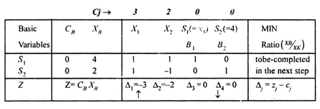
Write down the coefficients of all the variables in given LPP in the tabular form, as shown in table below to get an initial basic Feasible solution.
xB = B-1 b
The first row in table indicates the coefficient cj of variables in objective function, which remain same in successive tables. These values represent cost or profit per unit of objective function of each of the variables.
The second row gives major column headings for the simple table. Column CB gives the coefficients of the current basic variables in the objective function. Column xB gives the current values of the corresponding variables in the basic.
Number aij represent the rate at which resource (i- 1, 2- m) is consumed by each unit of an activity j (j = 1,2 … n).
The values zj represents the amount by which the value of objective function Z would be decreased or increased if one unit of given variable is added to the new solution.
It should be remembered that values of non-basic variables are always zero at each iteration.
So x1 = x2 = 0 here, column xB gives the values of basic variables in the first column.
So 5, = 4, s2 = 2, here; The complete starting feasible solution can be immediately read from table 2 as s1 = 4, s2, x, = 0, x2 = 0 and the value of the objective function is zero.
Step 3:
Test for optimality:
Now, proceed to test basic feasible for optimality by the rules given below. This is done by computing the “net evaluation” Dj for variable xj by the formula
Optimality Test:
(i) If all Δj ≥ 0, the solution under test will be optimal.
(ii) If at least one Δj is negative, the solution under test is not optimal, then proceed to improve the solution in step 4.
(iii) If corresponding to most negative Δj, all elements of the column Xj are negative or zero (≤ 0), then the solution under test will be unbounded
Applying this rule for testing the optimality of starting basic feasible solution, it is observed that Δ1, and Δ2 both are negative. Hence proceed to improve this solution in step 4.
Step 4:
In order to improve this basic feasible solution, the vector or entering the basis matrix and the vector to be removed from the basis matrix are determined by the following rules, such vectors are usually named as “incoming vector” and “outgoing vector” respectively.
“Incoming Vector”:
The incoming vector Xk is always selected corresponding to the most negative value of Δj. (say Δk). Here Δk = Mix (Δ1,Δ2) = Min [ – 3, -2] = – 3 = Δ.
Therefore k = 1 and column vector x1, must enter the basis matrix. The column x1 is marked by an upward arrow (↑).
“Outgoing Vector”:
The outgoing vector βr is selected corresponding to the minimum ratio of elements of XB by the corresponding positive elements of predetermined incoming vector XK. This rule is called the Minimum Ratio Rule. In mathematical form, this rule is written as,
Comparing both sides of this equation, r = 2 so the vector B2 marked with downward arrow (↓) should be removed from the basis matrix.
Now starting table (2) is modified to table (3)
Step 5:
In order to bring B2 in place of incoming vector X1 =
unity must occupy the marked ‘□’ position and zero at all other places of X1. If the number in the marked ‘□’ position is other than unity, divide all elements of that row by the ‘key element’ (the element at the intersection of minimum ratio arrow (←) and incoming vector arrow (↑) is called the key element). Then subtract appropriate multiples of this new row from the other remaining rows, so as to obtain zero in the remaining position of the column X1.
Thus, the process can be fortified by simple matrix transformation as follow:
The intermediate coefficient matrix is:
Table 4:
Now construct the improved simple table as follows:
From this table, the improved basic feasible solution is read as:
x1 = 2, x2 = 0, s1 = 2 , s2 = 0
The improved value of Z = 6
Thus the optimal solution is obtained as
xB = 3, x2 = 1, max z = 11
Step 6:
Now repeat step 3 through 5 as and when needed until an optimum solution is obtained in table 5.
Δk = Most negative Δj = – 5 = Δ2
... k = 2 and Hence X2 should be entering vector (Key column) By minimum ratio ratio
Since negative Ratio is not counted,] so the second ratio is not considered.
Since first ratio is minimum, remove the first vector p, form the basis matrix. Hence the key element is 2.
Developing the first Row by the key elements 2, the intermediate coefficient matrix is obtained as
This solution as read from this table is x1 = 3, x2 = 2, S1, = 0, S2 = 0 and Z= 11.
Also using the formula Δj = CB Xj – Cj verify that all Δj‘s are non-negative. Hence the optimum.
x1, = 3
x2 – 1
Max Z = 11
Simple Way for Simplex Computations:
Complete solution with its different computational steps can be more conveniently represented by a single table (6).
Thus the optimal solution is obtained as:
X1 = 3, x2 = 1, max z = 11
Example 2:
Minimize z=x2– 3x3 + 2x5
Subject to 3x2 – 23 + 2x5 ≤ 7
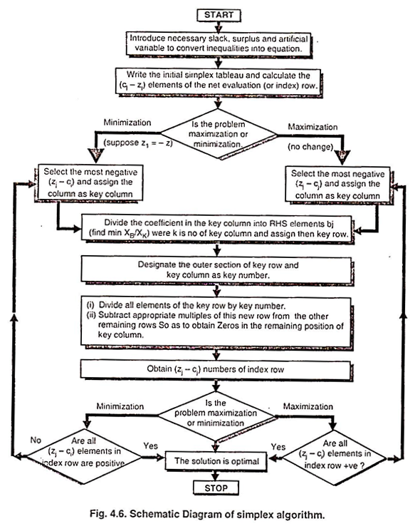
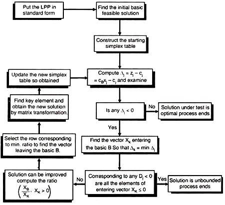
Schematic diagram of simplex Table:


